Why do you want to regularize input in deep learning?

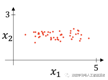
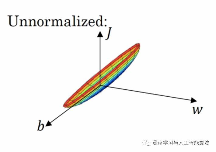
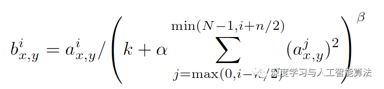
The author of this article is original, please indicate the source.

Today we're going to explore why input normalization—also known as standardization—is an essential step in many machine learning workflows.

Input normalization is essentially a form of local normalization, first introduced by Krizhevsky and Hinton in their groundbreaking ImageNet paper. It's a technique designed to standardize data across different dimensions and feature distributions.

In real-world applications, datasets often contain features with varying scales or distributions, which can make training models more challenging. Imagine working with data that looks something like this:

Such data can lead to inefficient gradient descent, where the optimization process becomes slow and unstable. Let’s visualize what the gradient descent landscape might look like for such data:

As you can see, it's a long and narrow three-dimensional shape. During backpropagation, if gradients start to diminish at both ends, the entire process can become very lengthy and inefficient. To address this issue, input normalization helps to stabilize and accelerate the training process.

Here's the formula used for input normalization:

Applying this normalization makes the gradient descent path much smoother, allowing for faster convergence regardless of the starting point:

Now, let's take a look at how this is implemented in TensorFlow. The relevant API is `tf.nn.local_response_normalization`, also known as `tf.nn.lrn`. Here's the function definition:

Local_response_normalization(input, depth_radius=5, bias=1, alpha=1, beta=0.5, name=None)

This function has several parameters: `input` is the tensor you want to normalize; `depth_radius` corresponds to n/2 in the formula; `bias` is an offset value; `alpha` is the scaling factor; and `beta` controls the exponent in the normalization formula.

In essence, LRN works by dividing each pixel by the sum of squared values of neighboring pixels within a specified radius. This helps to normalize the responses across channels, making the model more robust to variations in input.

Let's see how this works in practice with some code:

import numpy as np

import tensorflow as tf

a = 2 * np.ones([2, 2, 2, 3])

print(a)

b = tf.nn.local_response_normalization(a, 1, 0, 1, 1)

with tf.Session() as sess:

print(sess.run(b))

The output of 'a' is:

And the result after applying normalization (output 'b') is: