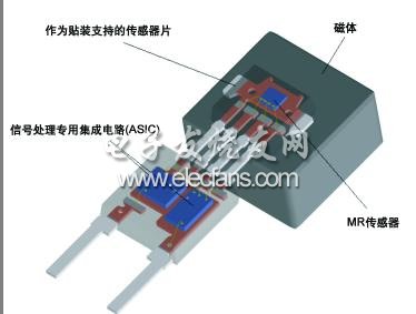
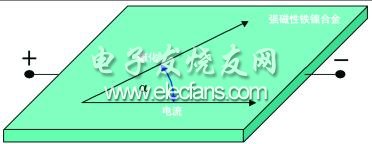
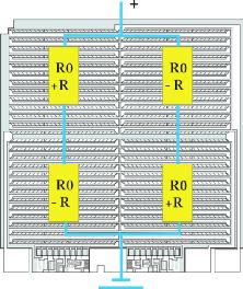
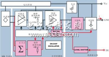
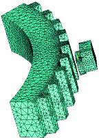
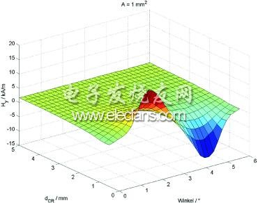
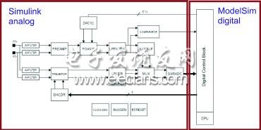
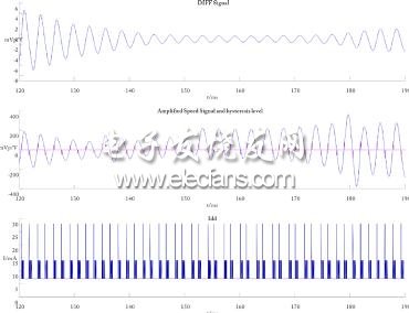
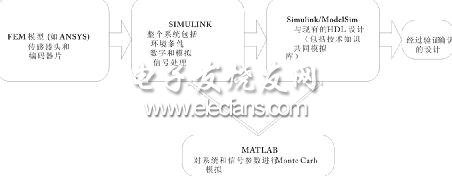
The magnetoresistance effect supports a variety of sensor applications in automobiles. Magnetoresistive sensors are primarily used to measure the speed and angle of mechanical systems. Thus, the magnetoresistive sensor becomes part of a complex system of electrical, magnetic, and mechanical components. Because all components affect the system's response, emulation of the entire system is important when planning the system and its operation. The following focuses on the modeling and simulation of such systems. This article refers to the address: http:// The mechanical design and selection of permanent magnets that generate magnetic fields can greatly affect the acquisition of measurement data. Therefore, it is important to use simulation techniques for in-depth analysis before deploying the entire system to ensure that the target functionality is achieved and costs are reduced. Therefore, the establishment of a system model in the early development process, which is then used to support the development of subsequent products, can also play an important role in solving such problems in the design process. The overall system modeling and simulation of the new speed sensor is discussed below. Figure 1 AMR sensor system consists of two packages Figure 2 Anisotropic magnetoresistance effect Signal Detection Modern sensor systems consist of two components—the basic sensor and the Signal Processing Application Specific Integrated Circuit (ASIC) (Figure 1). It has been shown that the anisotropic magnetoresistance effect discovered by Lord Klevin in 1857 is particularly suitable for detecting magnetic fields. First consider a ferromagnetic material that generally has a plurality of magnetic domain structures. These structures, called Weiss magnetic domains, have different internal magnetization directions from each other. If this material is tiled into a thin layer, the magnetization vector is in the planar direction of the material layer. In addition, it can be more accurately assumed that only one magnetic domain exists. When such an element is exposed to an external magnetic field, the latter changes the direction of the internal magnetization vector. If a current flows through the component at the same time, a resistance is generated (Figure 2), depending on the angle between the current and the magnetization. When the current and magnetization directions are at right angles to each other, the resistance is the smallest, and when the two are parallel, the resistance is maximum. The magnitude of the change in resistance depends on the material. The nature of the ferromagnetic material also determines the dependence on temperature. The best alloy with a maximum resistance change of 2.2% and good response to temperature changes is an alloy of 81% nickel and 19% iron. The basic sensors in all of NXP's sensor systems use this strong magnet nickel alloy. Several AMR resistors are individually configured in the Wheatstone bridge circuit to enhance the output signal and improve temperature response characteristics. This circuit can also be fine tuned during the manufacturing process. Figure 3 shows how to configure AMR components on the die. The device that determines the speed is mostly composed of two components: the encoder wheel and the sensor system. The encoder wheel can be active or passive. The drive wheel is magnetized so the MR sensor detects changes between the North and South poles. In the case of a passive wheel, the magnetization is replaced by a toothed structure. As shown in Figure 1, the sensor head must also have a permanent magnet for generating a magnetic field. Next, we will only discuss passive encoder wheels that are known for their extremely small tolerances. This does not cause any deflection of the magnetization vector of the AMR element when the sensor is symmetrically facing the gap between the teeth of one tooth or the passive wheel. When the external noise field is ignored and the bridge circuit is considered, the output signal gets a value of zero. However, if the sensor head is in front of the tooth edge, the magnetic input signal reaches an extreme value. The result of the function of the tooth/void or void/tooth switching type is very close to the minimum or maximum of the sinusoid of the magnetic input signal. Signal processing To determine the speed, the magnetic input signal is encoded into an electrical pulse train and is typically transmitted over the 7/14 mA protocol. In the simplest case, a comparator can be used to generate a pulse sequence. Hysteresis is typically added to the comparator circuit to eliminate the effects of low noise. However, such a Schmitt trigger does not ensure its functionality at high noise levels. For example, significant fluctuations in the gap between the sensor head and the encoder wheel can cause fluctuations in the amplitude of the magnetic input signal. If the amplitude becomes small, or even no longer exceeds or falls below the hysteresis threshold, the output signal remains in its last state of active operation regardless of the position of the encoder wheel. This change may occur at the distance between the sensor and the encoder wheel when detecting the speed in the ABS system. When there is a load change (such as a sudden steering action), the centrifugal force acting laterally on the wheel creates a bending moment on the axle. This will change the position of the encoder wheels mounted on the shaft associated with the sensor, which are combined with the wheel suspension. Magnetic displacement also affects the normal operation of the system. For example, the noise field can cause the actual measurement signal to be boosted or weakened, causing the critical value of the Schmitt trigger to be overestimated or underestimated. However, the displacement is not only caused by the external field. The extremely high speed of the passive wheel creates eddy currents in the wheel, which in turn creates a magnetic noise field. The resulting displacement can affect the reliability of the operation. To eliminate the effects of this noise on the output signal, a signal processing application specific integrated circuit (ASIC) is incorporated into the other package. The latter also includes a line driver to provide supply voltage for signal processing and high voltage interfaces (Figure 1). Figure 4 shows the signal processing architecture. The central components used for troubleshooting are tuned amplifiers, offset cancellation circuits, and smart comparators. Depending on the distance between the sensor and the encoder wheel, the adjustable amplifier can be matched to the signal level. For offset cancellation circuits, there is a control system (unlike a high-pass filter) that eliminates offset while maintaining the system frequency at 0 Hz. Otherwise, it is impossible to detect an encoder wheel that stops moving. The critical value of the intelligent comparator is variable and can be set such that the hysteresis is between 20% and 45% of the signal amplitude. This ensures that noise is adequately suppressed and that a 50% amplitude dip does not affect the normal operation of the system. The individual component control of the analog front end is implemented via a digital interface. The systems are all developed and validated using simulation techniques. The system development is outlined below, along with an explanation of how to use the model to improve the design. Figure 3 AMR component configuration on the die Figure 4 Signal processing principle of modern speed sensor Figure 5 Grid - starting point system simulation of magnetic field finite element simulation To develop a sensor system, you must first have an overall understanding of the expected magnetic input signal. The first step is to understand the standard specifications of the permanent magnets on the encoder wheel and sensor head, as well as the expected dimensions and tolerances. The magnetic field is determined by FEM simulation with the ANSYS method. There is a problem with modeling the encoder wheel, sensor elements and magnets (Figure 5). The strength of the magnetic field as a function of this can then be determined from the distance between the sensor element and the encoder wheel. Figure 6 is a three-dimensional illustration of the magnetic input signal on the sensor bridge as a function of distance. It is easy to see that the input signal is sinusoidal and the amplitude of the signal decreases significantly with increasing distance. In addition to the distance, the positional deviation also causes the amplitude to decrease. For example, if the sensor head is not at the center of the front of the encoder wheel, the signal amplitude will also decrease. According to the FEM simulation method, this also converts the mechanical specification into the expected magnetic variable. Unlike air gap changes, tilt can cause an offset, which can also affect the normal operation of the system. FEM simulation can also predict its effects (Figure 7), and the results can be directly translated into allowable position tolerances. After determining the magnetic field is the sensor system simulation. The change in resistance of the AMR component is a direct result of the anisotropic magnetoresistance effect. Thus, the result of the magnetic field simulation results in a change in the resistance of the input signal representing the signal processing. Modeling the analog front end can be done using Simulink. This behavioral model is the product of conceptual design and marks the starting point for product development. Each Simulink block corresponds to an analog signal processing component, such as an amplifier or filter. However, the control portion of the analog component has not been considered, which is implemented by a digital system. The HDL design simulates the functions implemented digitally and is finally formed after product development. Therefore, the overall system simulation is Simulink's behavioral model for analog components and ModelSim's common simulation for HDL design (Figure 8). A smooth transition from the concept phase to the HDL design and subsequent phases can be achieved through simulation. In co-simulation, the Simulink reference model can be gradually replaced with Verilog code deployed in ModelSim to validate the HDL design item by item. This process can continue until the entire digital part is implemented in Verilog, while the analog system components remain as Simulink models. This tool combination has also proven to be equally useful for IC evaluation. Using this tool from start to finish makes it easier to understand IC behavior and create a framework for analyzing and interpreting any errors. The main benefits of these tools are the ability to respond to customer inquiries more quickly and accurately, and to better understand sensor functions related to environmental conditions. Figure 6 Simulation of magnetic input signal as a function of sensor head and encoder wheel distance Figure 7 shows the calculation of the magnetic field for determining the allowable position tolerance Figure 8 Simulation of the simulation of the front end and the digital block Through this modeling, you can analyze the behavior of the system as a function of the input signal. The first chart in Figure 9 shows the magnetic input signal produced by changing the distance between the sensor and the encoder wheel. This signal is the result of a finite element simulation, after which the AMR effect converts this signal into the electrical output signal of the sensor bridge. The middle chart is the result of analog signal processing. The next chart shows the output signal. This device uses the A 7/14/28 mA protocol. This protocol can be used to convey additional information, such as sensing rotation or air gap length. In addition to these results, you can also check the operation of the digital controls. Figure 10 shows an example of a signal image in ModelSim. Simulation control with MATLAB combined with other simulators creates more options. First, for example, the simulation can be automated. Signal simulation can then be performed in MATLAB using a number of algorithms. For example, Monte Carlo simulation of the required system and signal parameters followed by automated analysis. With FEM simulators (such as NASYS), you can extend the system components you emulate, even the MR sensor heads and associated encoders, extending the system view to directly related areas around the sensor. Figure 11 shows the entire tool chain for this purpose. Figure 9 Simulation results: electrical output signal comparison magnetic input signal Figure 10 Simulation of digital system components Figure 11 complete simulation chain to sum up A magnetic field simulator is used to determine the magnetic input signal, while Simulink simulates the analog input. Digital control simulation of analog components after HDL design. Finally, the entire system is fully simulated. Modeling has become part of pre-development and is continually being optimized as the product development process progresses. Finally, a design that is validated to meet product specifications and a model that can be used to solve subsequent problems is included as part of the market support.
FTTH Fiber Optic Socket Terminal Box, fiber termination box provides a mini density wall-mounted solution for next generation networks, which aims to provide and manage minimum numbers of fibers in a limited space.
It is normally installed in the way of wall-mounted. Widely used in FTTH access network, telecommunication networks, CATV networks, data communications network, local area networks, indoor and outdoor application.
Mini FTTH terminal box is designed specially for FTTx application, which suits for jointing fibers pigtail and it protects fiber optic splices and helps to share out the connectivity to individual customers. Optical Termination Box is designed to connect raiser/distribution cables to subscriber`s drop cable in FTTx networks. It has 1 input port and 1 output ports on the bottom and it is easy to install on the wall.
FTTH Fiber Optic Socket Terminal Box Optical Fiber Terminal Box,Fiber Access Termination Box,Fiber Optic Terminal Box,Fiber Optic Junction Box,Fiber Optic Cable Junction Box Sijee Optical Communication Technology Co.,Ltd , https://www.sijee-optical.com